Have you ever wanted to show data from one spreadsheet inside another spreadsheet in Excel or Google Sheets? I often times analyze data for my clients where the same column of data is in two sheets, and I want to build a data relationship to show key performance indicators (KPIs) from the two datasets.
In this post, I will show you how to use VLOOKUP to link data between sheets.
Prerequisites To Follow This VLOOKUP Tutorial
You must have two sheets with data where one column is in both sheets. This like data is the key for our relationship between the two data sets. The key unlocks the data between the two sheets so we can build meaningful metrics and KPIs.
Here is a link to my own data sheet you can use for this tutorial:
Understanding VLOOKUP: What It is and How It Works
VLOOKUP is an Excel and Google Sheet function you can use to relate data between two sheets. All you need is the same column of data in both sheets. This like data is called a “key” and is used to build that relationship between data sets.
Have you ever had a “Master” spreadsheet with all your data? If so, then you probably know that the master sheet is the king of the castle. You don’t touch this master data, manually edit it, or massage it. You leave it alone!
But what if you need to create new data based on your “Master” spreadsheet? Well, thats where VLOOKUP comes into play.
What Is The Syntax For VLOOKUP?
VLOOKUP takes four arguments. They are:
- The single cell value (like A2) in Sheet2 you want to find in Sheet1 somewhere
- The entire range of data in Sheet1
- The column number (Column A would be number 1) you want to return in Sheet2
- The sorted argument Indicates whether the column you want to search for the primary key is sorted, in which case the closest match for search_key will be returned.
=VLOOKUP(
    A2,           // In Sheet2, the value in cell B2 (the data key) that you want to find in Sheet1.
    'Sheet1'!A:J, // The range of data in the Sheet1, where column A contains the lookup values (Keywords), and columns B through J contain the related data.
    4,            // The 4th column in the range, which contains the data you want to bring back (e.g., "Keyword Difficulty").
    FALSE         // Use FALSE to find an exact match for the value in B2. This works best when the keyword data is unique.
)
Pro Tip: When using VLOOKUP with the FALSE argument (exact match), the function will always return the first matching instance it finds in your lookup range, searching from top to bottom. While this behavior is consistent and predictable, it’s important to understand that if your lookup column contains duplicate keys, you might not be seeing all possible matches. For the most reliable data analysis, it’s generally best to work with unique keys. If you must work with duplicate keys, consider using more advanced functions like INDEX/MATCH combinations or FILTER to see all matching values.
How To Setup Your Data To Run VLOOKUP
Step 1 – In either Google Sheets or Excel create a dataset in Sheet1 with 5 columns. The first column will be our primary key. I am going to use SECompetitorO data for this example, but you can create whatever data you would like.
The columns will be:
- Keyword (The primary key, unique values with no duplicates)
- Domain
- Page
- Rank
- Difficulty
Step 2 – Create a second sheet with the following columns
- Keyword (The primary key, copy and paste the data from Sheet1 to create the relationship)
- Competitor
- Rank
- Page
Step 3 – Populate your two sheets with Data. Make sure the first column in each sheet contains your primary key.
Why You Should Use The VLOOKUP Formula
Our goal is to work smart, not hard, by pulling data from Sheet1 into Sheet2.
Sheet2 will hold new information not found in Sheet1 and two columns of data pulled over from Sheet1.
We can use the VLOOKUP formula to dynamically bring those two specific data columns from Sheet1 into Sheet2.
This ensures Sheet2 has both the fresh data and the linked columns from Sheet1, all without us having to manually copy anything. The formulas keep everything synced up automatically, so Sheet2 always displays the most current information from those two columns in Sheet1.
The benefits of this approach are:
- Formulas link the sheets so the Sheet1 columns in Sheet2 auto-update
- No need to repeatedly copy data by hand from Sheet1 to Sheet2
- Sheet2 contains its own new data plus always-updated data from Sheet1
- You can update Sheet1 without having to update Sheet2 because Sheet2 is dynamic!
How To Build The VLOOKUP Formula
We are going to pull the Rank and Page data from Sheet1 and dynamically populate the Rank and Page columns in Sheet2. The steps below work with the tutorial data below. If you are using your own data, you may have to make a few minor changes.
Here is the link to the tutorial data one more time:
steps to implement the VLOOKUP Formula:
- Open up the tutorial data in Google Sheets and click into Sheet2.
- Find column titles “Rank”.
- In the first empty cell, enter this formula
=VLOOKUP(A2,Sheet1!1:1000,4,FALSE)Notice that the third argument is the number 4. That’s because we are referencing column 4 in Sheet1 to access an pull in our data.
It should look like this:
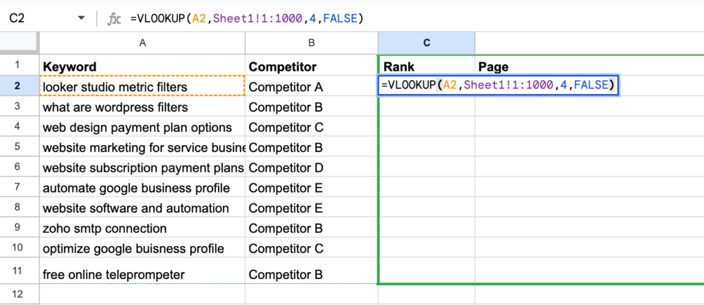
You should see the number 5 returned if you are using the sample data.
Next follow these steps to finish implementing the VLOOKUP formula:
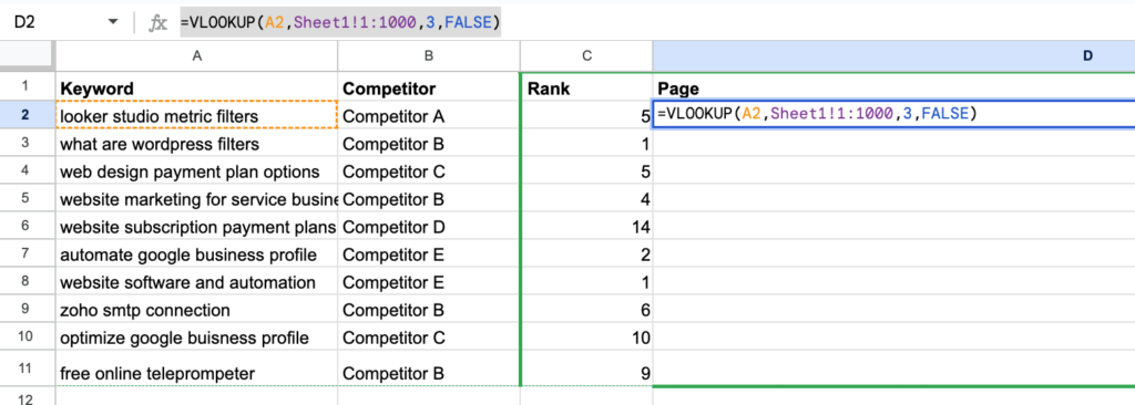
- Drag the formula down through the remaining cells in the Rank Column
- Find the Page column and enter this formula
=VLOOKUP(A2,Sheet1!1:1000,3,FALSE)Notice that the third argument is the number 3. That’s because we are referencing column 3 in Sheet1 to access an pull in our data.
You can drag this formula down through the remaining cells in the Page column.
It should look like this:
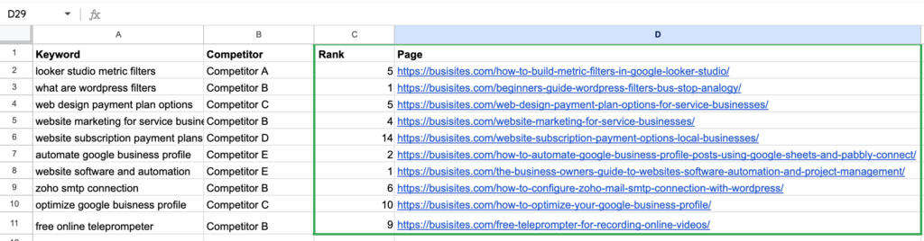
After you enter the formula, the sheet should look something like this:
Common Mistakes to Avoid When Using VLOOKUP
VLOOKUP is not an easy formula to master. It has taken me a long time to get comfortable with how the function works and what arguments its looking for. Review this list if you are having trouble getting your VLOOKUP formula to work:
Incorrect Column Index
Make sure the column index number is right. Remember, VLOOKUP counts columns from left to right, starting at 1 for the first column in your range.
Inadequate Range Selection
Choose the full range needed for your lookup. This includes the column with the lookup value and all the columns you want to pull data from.
Mishandling of Spaces and Characters
Extra spaces or hidden characters can mess up VLOOKUP. Use the TRIM function to eliminate extra spaces:
=VLOOKUP(TRIM(lookup_value), range, column_index, FALSE)If there are spaces in the lookup column, consider using INDEX-MATCH with TRIM instead.
Incorrect “is_sorted” Argument
When your data isn’t sorted, always set the last VLOOKUP argument to FALSE for exact matches. If you leave it out, VLOOKUP assumes TRUE, which can give you the wrong results with unsorted data.
Number Formatting Issues
Ensure that the numbers in your lookup value and the lookup range are formatted the same way. Numbers stored as text can cause errors. To fix this, use the “Convert to Number” option or wrap your lookup value in the VALUE function.
Lookup Value Exceeds Character Limit
VLOOKUP can’t handle lookup values longer than 255 characters. If you have longer values, switch to using INDEX-MATCH instead.
Incorrect File Path for External References
When pulling data from another workbook, make sure to include the full path. This means including the workbook name, sheet name, and range.
Frequently Asked Questions
What is VLOOKUP and how does it work in Google Sheets?
VLOOKUP is a function in Excel and Google Sheets that allows you to relate data between two sheets by searching for a value in one sheet and returning a corresponding value from another column. It requires a common key column in both sheets to establish the relationship and dynamically pull data, such as KPIs, without manual copying.
How do I set up my data for using VLOOKUP in Google Sheets?
To set up your data for VLOOKUP, ensure you have two sheets with a common key column. In Sheet1, organize your data with the primary key in the first column followed by the data you want to retrieve. In Sheet2, include the primary key and use the VLOOKUP formula to dynamically pull the desired columns from Sheet1. Make sure both sheets have consistent formatting and unique keys.
What are common mistakes to avoid when using VLOOKUP?
Common mistakes when using VLOOKUP include using an incorrect column index, selecting an inadequate range, mishandling spaces and characters, setting the wrong ‘is_sorted’ argument, having inconsistent number formatting, exceeding the character limit for lookup values, and providing incorrect file paths for external references. Ensuring these aspects are correctly handled will lead to more reliable results.
How can I handle extra spaces or hidden characters when using VLOOKUP?
Extra spaces or hidden characters can cause VLOOKUP to fail. To handle this, use the TRIM function to remove excess spaces from your lookup values. For example, use =VLOOKUP(TRIM(lookup_value), range, column_index, FALSE). If spaces are present in the lookup column, consider using INDEX-MATCH with TRIM for more reliable results.
What should I do if my lookup value exceeds the character limit in VLOOKUP?
VLOOKUP has a 255-character limit for lookup values. If your lookup value exceeds this limit, switch to using the INDEX-MATCH combination instead. INDEX-MATCH does not have the same character limitations and can handle longer lookup values effectively.
Wrapping Up
Understanding how to use VLOOKUP effectively transforms the way you handle data relationships in spreadsheets. By creating dynamic connections between your sheets, you eliminate the tedious task of manual data entry and reduce the risk of errors that come with copying and pasting. This powerful function not only saves you valuable time but also ensures your data stays consistently updated across all your sheets.
Remember, the key to successful VLOOKUP implementation lies in maintaining clean data with unique keys in your master sheet and understanding how the four arguments work together. Whether you’re analyzing customer data, tracking inventory, or building complex KPI dashboards, VLOOKUP serves as an essential tool in your spreadsheet toolkit.
Start implementing these techniques in your own spreadsheets today, and you’ll discover just how much more efficient your data management can become. For more advanced spreadsheet tutorials and data analysis tips, don’t forget to bookmark our blog and subscribe to our YouTube channel.